Riemann Sum

Before plunging into the detailed definition of the integral, we outline the main ideas.

First, the region under the curve is divided into infinitely many vertical strips of infinitesimal width dx. Next, each vertical strip is replaced by a vertical rectangle of height f(x), base dx, and area f(x) dx. The next step is to form the sum of the areas of all these rectangles, called the infinite Riemann sum (look ahead to Figures 4.1.3 and 4.1.11). Finally, the integral is defined as the standard part of the infinite Riemann sum.

	If want to get more experience with Riemann sums, you should download the Riemann sum simulation from the Learning by Simulations site.

The infinite Riemann sum, being a sum of rectangles, has an infinitesimal error. This error is removed by taking the standard part to form the integral.

It is often difficult to compute an infinite Riemann sum, since it is a sum of infinitely many infinitesimal rectangles. We shall first study finite Riemann sums, which can easily be computed on a hand calculator.

Suppose we slice the region under the curve between a and b into thin vertical strips of equal width. If there are n slices, each slice will have width ∆x = (b - a)/n. The interval [a, b] will be partitioned into n subintervals

where

The points x₀, x₁,..., x_n are called partition points. On each subinterval [x_k-1, x_k], we form the rectangle of height f(x_k-1). The kth rectangle will have area

From Figure 4.1.3, we can see that the sum of the areas of all these rectangles will be fairly close to the area under the curve. This sum is called a Riemann sum and is equal to

It is the area of the shaded region in the picture. A convenient way of writing Riemann sums is the "Σ-notation" (Σ is the capital Greek letter sigma),

Figure 4.1.3 The Riemann Sum

The a and b indicate that the first subinterval begins at a and the last subinterval ends at b.

We can carry out the same process even when the subinterval length Δx does not divide evenly into the interval length b-a. But then, as Figure 4.1.4 shows, there will be a remainder left over at the end of the interval [a, b], and the Riemann sum will have an extra rectangle whose width is this remainder. We let n be the largest integer such that

a + n Δx ≤ b,

and we consider the subintervals

[x₀, x₁],..., [x_n-₁, x_n], [x_n, b],

where the partition points are

x₀ = a, x₁ = a + Δx, x₂ = a + 2 Δx,..., x_n = a + n Δx, b.

Figure 4.1.4

x_n will be less than or equal to b but x_n + ∆x will be greater than b. Then we define the Riemann sum to be the sum

Thus given the function f, the interval [a, b], and the real number ∆x > 0, we have defined the Riemann sum. We repeat the definition more concisely.

If x_n = b, the last term f(x_n)(b - x_n) is zero. The Riemann sum is a real function of three variables a, b, and Δx,

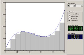
The symbol x which appears in the expression is called a dummy variable (or bound variable), because the value of f (x) Δx does not depend on x. The dummy variable allows us to use more compact notation, writing f(x)∆x just once instead of writing f(x₀)∆x, f(x₁) ∆x, f(x₂) ∆x, and so on.

From Figure 4.1.5 it is plausible that by making ∆x smaller we can get the Riemann sum as close to the area as we wish.

Figure 4.1.5

The Riemann sum and the area of a triangle.

The Riemann sum and the area of a semicircle.