 You are working with the text-only light edition of "H.Lohninger: Teach/Me Data Analysis, Springer-Verlag, Berlin-New York-Tokyo, 1999. ISBN 3-540-14743-8". Click here for further information.
| You are working with the text-only light edition of "H.Lohninger: Teach/Me Data Analysis, Springer-Verlag, Berlin-New York-Tokyo, 1999. ISBN 3-540-14743-8". Click here for further information.
|
Table of Contents  Statistical Tests Comparing Distributions Chi-Square Test Statistical Tests Comparing Distributions Chi-Square Test |
|
| See also: survey on statistical tests, Kolmogorov-Smirnov test, tests for normality, distribution calculator |   |

The easiest way to compare distributions is to compare them visually.
We overlay a histogram of the data with the theoretical distribution with
which it is to be compared. Of course this approach lacks statistical justification.
A sound method to compare empirical and known (parametric) distribution
is the ![]() -test.
-test.
One practical problem is that the evaluation of parametric distribution functions results in probabilities instead of frequencies. In order to compare the empirical and theoretical distribution we have to to estimate the expected frequencies by multiplying the theoretical probabilities by the number of samples.

The probability that the variable falls into a bin [ai,ai+1] is the difference of the probabilities of x being less than the bin boundaries ai and ai+1, respectively: Prob(ai < x < ai+1) = Prob(x < ai+1) - Prob(x < ai)
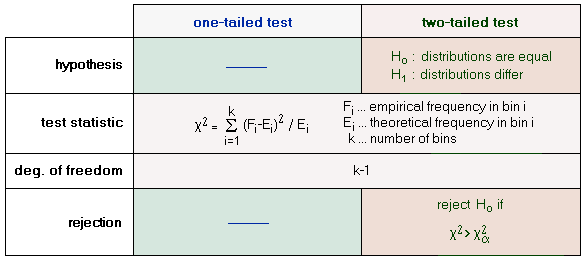
For each bin, the squared difference between the frequencies of the
empirical and the theoretical distribution are calculated. The squared
differences are divided by the expected frequencies. The sum of these relative
or weighted squared differences is the ![]() statistic. The null hypothesis is that the two distributions are the same,
and the differences are due to random errors.
statistic. The null hypothesis is that the two distributions are the same,
and the differences are due to random errors.
| Note: | Another important point to remember is that the theoretical probabilities
are normally tabulated for standard parameters, i.e. zero mean and unit
variance for the normal distribution. So we either have to standardize
the histogram, or estimate the distribution parameters and use them for
the calculation of the probabilities in the appropriate bins of the histogram.
The number of estimated parameters k has an influence on the degree of
freedom used in the |
Last Update: 2005-Jul-16